
Introduction: The Worldwide Biocracy
1. Intellectual Hierarchy in Canada
2. Intellectual Hierarchy in Brazil
3. Intellectual Hierarchy in England
4. Intellectual Hierarchy in The Netherlands
5. Intellectual Hierarchy in the United States
6. Intellectual Hierarchy in Australia
7. Intellectual Hierarchy in Africa
8. Intellectual Hierarchy in Southeast Asia
Conclusion
Introduction
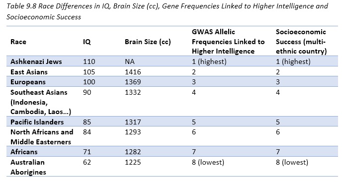
No matter the multi-ethnic country in the world, the hierarchy in social stratification remains essentially the same, with an order dictated by the racial IQ:
- Ashkenazi Jews (110)
- East Asians (105)
- Europeans (100)
- Southeast Asians (92)
- Arctic People (91)
- European-African hybrids (81-90)
- Native Americans (86)
- North African and South Asian (84-88)
- Africans (71-80)
- Australian Aborigines (62)
The differences are, of course, more marked between the races whose IQ differs appreciably and are more tenuous between the races of near intelligence.
This hierarchy is reflected in:
- Education
- Average wages
- Crime rate (inversely proportional to IQ)
- Socio-economic status
- Fertility (inversely proportional to IQ). However, there are exceptions to this fertility rate, showing the place of certain cultural factors, such as the high fertility rate of Hispanics of the Catholic religion.
- Mental retardation (increases while IQ decreases)
- Academic achievement
- Juvenile delinquency (increases while IQ decreases)
- The percentage of single mothers increases while IQ decreases.
- Unemployment rate (increases while IQ decreases)
- Success at the SAT (the entrance test of most American universities)
- The prevalence of talented people.
These differences all derive from the intellectual inequalities between the races/populations of homo sapiens. Ashkenazi Jews, East Asians and Europeans (the First World) are genetically more intelligent, distinguished by higher rates of cultural achievement, higher wages, lower crime rate, higher socio-economic status, lower fertility rate, good academic achievements, low juvenile delinquency, low single mothers rate, limited unemployment rate, high THS achievement and high prevalence of gifted individuals.
Conversely, North Africans, Middle Easterners, Africans and Aborigines in Australia are characterized by lower intellectual ability, and as a result they reach lower education level, they get lower wages, they have a higher crime rate, lower socio-economic status, higher fertility, lower academic achievement with more juvenile disorders, a high percentage of single mothers, high unemployment, lower SAT scores, and lower gifted prevalence.
All data below are taken from ‘The global bell curve‘ (2008), Richard Lynn.
This unchanged hierarchy is the consequence of the highly genetic causality of intelligence. Regardless of the country, populations with a higher frequency of high intelligence alleles (Ashkenazi Jews, East Asians, Europeans) are better off than less intelligent populations with lower frequency of these alleles for a high intelligence and a smaller and less powerful brain (North African, Middle Easterners, African and Australian aborigines).
1. Intellectual Hierarchy in Canada
Table 6.7. IQs of Races in Canada
| Group | Jews | Chinese | Whites | Inuits | Native Americans | Blacks |
|---|---|---|---|---|---|---|
| IQ | 109 | 101 | 100 | 91 | 87 | 84 |
1.1 The Hierarchy Remains Determined by IQ for Education
Table 6.8. Race and ethnic differences in educational attainment
| Measure | Year | Jews | Chinese | British | French | European | Native American | Black | |
| 1 | Illiterate % | 1921 | 7 | 27 | 1 | 8 | 14 | – | 8 |
| 2 | Illiterate % | 1931 | 4 | 15 | 1 | 6 | 8 | – | 8 |
| 3 | 10th grade % | 1951 | 53 | 31 | 55 | 30 | 35 | 6 | – |
| 4 | 10th grade % | 1961 | 64 | 45 | 63 | 38 | 31 | 9 | – |
| 5 | 10th grade % | 1971 | 80 | 75 | 77 | 59 | 58 | 38 | – |
| 6 | 10th grade % | 1981 | 85 | 80 | 84 | 77 | 72 | 55 | 88 |
| 7 | Years-NB | 1981 | 13.5 | 13.1 | 11.7 | 11.1 | 11.9 | – | 11.8 |
| 8 | Years-FB | 1981 | 12.7 | 11.9 | 12.7 | 12.4 | 10.7 | – | 12.4 |
| 9 | Years-M | 1991 | 15.0 | 14.7 | 12.3 | 11.7 | 12.4 | 9.5 | 12.8 |
| 10 | Years-W | 1991 | 14.6 | 14.6 | 12.6 | 12.2 | 12.5 | 10.4 | 13.0 |
| Sources: rows 1-6: Herberg, 1990b; rows 7-8: Li, 1988; rows 9-10: Sweetman & Dicks, 2000. | |||||||||
1.2 The Hierarchy Remains Determined by IQ for the Salaries
Table 6.11. Race and ethnic differences in annual earnings, 1941-2001
| Year | Jews | Chinese | British | French | European | Native American |
Black | Southeast Asian |
|
| 1 | 1941 | 1,327 | 931 | 1,515 | 1,007 | 1,115 | 802 | – | – |
| 2 | 1951 | 2,619 | 2,100 | 2,481 | 2,150 | 2,232 | 1,404 | – | – |
| 3 | 1961 | 7,426 | 3,895 | 4,852 | 3,872 | 3,319 | – | – | – |
| 4 | 1971 | 12,368 | 6,668 | 8,500 | 7,307 | 7,846 | – | – | |
| 5 | 1981 | 21,349 | 13,292 | 15,100 | 13,831 | 13,367 | 9,032 | 13,029 | – |
| 6 | 1991 | 50,100 | 34,570 | 34,660 | 31,615 | 33,100 | 27,535 | 28,495 | 35,615 |
| 7 | 2001 | 73,928 | 40,817 | 43,398 | – | – | 32,176 | 35,100 | 34,100 |
| Sources: 1941-1981: Herberg (1990b). 1981-2001: Statistics Canada. | |||||||||
1.3 Inverse Relationship between IQ and Crime Rates
Table 6.16. Race differences in crime (per 1,000 population)
| Year | Sex | White | Black | Indian | South Asian | Chinese |
| 1992 | M/F | 7.1 | 36.9 | 19.9 | 4.6 | 3.5 |
2. Intellectual Hierarchy in Brazil
Table 4.2. Race and Ethnic Differences in Intelligence in Brazil
| Group | Japanese | Europeans | Mulattos | Blacks | Reference |
|---|---|---|---|---|---|
| IQ | 99 | 95 | 81 | 71 | Fernandez, 2001 |
| Numbers | 186 | 735 | 718 | 223 |
2.1 Hierarchy Remains Determined by IQ for Education
Table 4.3. Race and ethnic differences in educational attainment and literacy (percentages)
| Measure | Year | japanese | Whites | Mulattos | Blacks | |
| 1 | High school | 1950 | – | 4.9 | 0.5 | 0.2 |
| 2 | Literate | 1950 | – | 59.3 | 31.1 | 26.7 |
| 3 | Degree | 1980 | 10.0 | 6.4 | 1.9 | 1.0 |
| 4 | Literate | 1991 | – | 84.3 | 66.6 | 65.3 |
| 5 | High school-M | 1996 | – | 56.5 | 39.3 | 28.0 |
| 6 | High school-F | 1996 | – | 64.9 | 48.1 | 45.4 |
| 7 | Literate | 1999 | – | 91.7 | 80.4 | 79.0 |
| 8 | Degree | 1996 | – | 10.0 | 2.4 | 1.8 |
2.2 Hierarchy Remains Determined by IQ for Salaries and Socioeconomic Status
Table 4.4. Race and ethnic differences in earnings and socioeconomic status
| Measure | japanese | Europeans | Mulattos | Blacks | |
| 1 | Income, 1960 | – | 11,601 | 6,492 | 5,444 |
| 2 | Income, 1980 | 35,610 | 21,867 | 11,053 | 9,004 |
| 3 | Income, 1991 | – | 224,752 | 132,400 | 129,165 |
| 4 | Poverty, 1987 | – | 24% | 44% | 46% |
| 5 | Professionals, 1950 | – | 4.5% | 2.4% | 2.1% |
| 6 | Professionals, 1980 | – | 9.0% | 3.8% | 2.5% |
| 7 | Professionals, 1991 | – | 27.5% | 15.8% | 12.1% |
| 8 | Unemployment: M | – | 3.5% | 4.1% | 4.8% |
| 9 | Unemployment: F | – | 3.3% | 3.6% | 4.4% |
| Sources: 1: Marx, 1998; 2-3, 6-7: Lovell, 1993; 4-5 Andrews, 1992; 8-9: PNAD, 1997 | |||||
2.3 Inverse Relationship between IQ and Crime Rates
Table 4. 10. Percentages of races in population and convictions for homicide, 2003
| Race | % Population | % Homicide |
| White | 53 | 39.7 |
| Mulatto | 40 | 49.9 |
| Blacks | 6 | 9.8 |
| Asians | 1 | 0.4 |
2.4 About Mothers
Table 4.12 Race differences among mothers in Rio de Janeiro in 2000
| Measure | Whites | Mulattos | Blacks |
| Age <20 years | 16.3 | 22.3 | 24.5 |
| Education <4 years | 5.8 | 10.6 | 13.9 |
| Higher education | 13.1 | 2.8 | 1.3 |
| Smoked while pregnant | 10.3 | 14.9 | 18.5 |
| Baby syphilitic | 0.8 | 1.9 | 3.0 |
3. Intellectual Hierarchy in England
Table 4. Race Differences in Intelligence in England
| Group | Jews | Asians | Whites | South Asians* | Blacks |
|---|---|---|---|---|---|
| IQ | 110 | 105 | 100 | 92 | 86 |
*South Asians = Pakistanis, Bangladeshis, Indians.
3.1 Racial Composition of England (Tables 5.1 and 5.2)
Table 5. Number of non-Europeans in England, 1951-2001
| Year | Blacks | Indians | Pak./Ban. | Chinese |
| 1951 | 16,000 | 111,000 | 11,000 | – |
| 1961 | 172,000 | 157,000 | 31,000 | – |
| 1971 | 302,000 | 313,000 | 136,000 | – |
| 1991 | 890,000 | 840,000 | 640,000 | 157,000 |
| 2001 | 1,100,000 | 1,100,00 | 1,000,000 | 209,000 |
Table 5. Race and Proportion of the English Population
| Year | Whites | Blacks | Indians | Pak./Ban. | Chinese |
| 1991 | 94.5 | 1.6 | 1.5 | 1.2 | 0.3 |
| 2001 | 92.4 | 2.1 | 1.9 | 1.4 | 0.4 |
3.2 Hierarchy Remains Determined by IQ for Salaries
Average weekly earnings of racial groups
| Year | White | Black | Indian | Pak./Ban. | Chinese | |
| 1 | 1994 | 331 | 311 | 317 | 220 | 368 |
| 2 | 1995 | 309 | 268 | 279 | 230 | 342 |
| 3 | 2001 | 332 | 225 | 327 | 182 | – |
3.3 Inverse Relation between IQ and Crime Rates
Table 5. 7. Incidence of mental retardation and backwardness (percentage)
| Date | Condition | Whites | Blacks | S. Asians | |
| 1 | 1970 | Retardation | 0.68 | 2.33 | 0.40 |
| 2 | 1972 | Retardation | 0.66 | 2.90 | – |
| 3 | 1980 | Backwardness | 8.00 | 19.00 | 12.00 |
3.4 Hierarchy Remains Determined by IQ for Education (table 5.8, 5.9, and 5.10)
Table 5.8. Race differences in educational attainment at age 7 (percentage passes)
| Group | Reading | Writing | Arithmetic |
| Chinese | 90 | 88 | 96 |
| Whites | 85 | 82 | 91 |
| Mixed | 85 | 82 | 91 |
| Asians | 80 | 78 | 86 |
| Blacks | 78 | 74 | 84 |
Table 5.9. Race differences in educational attainment (Percentage passes)
| Age 11 | Age 14 | |||||
| Group | English | Math | Science | English | Math | Science |
| Chinese | 82 | 88 | 90 | 80 | 90 | 82 |
| Whites | 76 | 73 | 87 | 70 | 72 | 70 |
| Mixed | 77 | 72 | 87 | 69 | 69 | 67 |
| Asians | 69 | 67 | 79 | 66 | 66 | 59 |
| Blacks | 68 | 60 | 77 | 56 | 54 | 51 |
Table 5. 10. Race differences in educational attainment for 11-year-olds (percentage)
| Group | N | English | Math | Science |
| jews | 905 | 92 | 91 | 95 |
| Chinese | 1,938 | 81 | 89 | 89 |
| Whites | 489,887 | 78 | 74 | 87 |
| South Asians | 38,721 | 74 | 69 | 79 |
| Indian | 12,725 | 83 | 80 | 87 |
| Pakistani | 16,307 | 68 | 61 | 72 |
| Bangladeshi | 5,979 | 71 | 66 | 77 |
| Other Asian | 3,710 | 75 | 77 | 82 |
| Blacks | 21,575 | 70 | 63 | 77 |
| Caribbean | 8,739 | 70 | 61 | 78 |
| African | 10,617 | 69 | 64 | 75 |
| Other Blacks | 2,219 | 71 | 64 | 80 |
| Others | 4,804 | 66 | 70 | 76 |
| Unclassified | 18,530 | 71 | 68 | 81 |
| Total | 592,163 | 77 | 73 | 86 |
3.5 Inverse Relation between IQ and Delinquency
Table 5. 19. Race differences in conduct disorders in children (odds ratios)
| Sex | White | Black | Chinese | S. Asian | |
| 1 | M/F | 1.0 | 1.4 | ||
| 2 | M | 1.0 | 3.9 | ||
| 3 | F | 1.0 | 2.3 | – | ? |
| 4 | M/F | 1.0 | 4.4 | 0.18 | 0.92 |
| Sources: 1: Goodman & Richards, 1995; 2-3: Tizard et al., 1988; 4: Gillborn and Gipps, 1996. | |||||
3.6 Inverse Relation between IQ and Crime Rates
Table 5.20. Race différences in crime (odds ratios)
| Year | Sex | White | Black | Indian | Pak./Ban. | Chinese | |
| 1 | 1993 | M | 1.00 | 6.10 | 0.87 | 0.87 | ? |
| 2 | 1995 | M | 0.88 | 7.12 | 0.87 | 1.42 | 0.66 |
| 3 | 1995 | F | 0.80 | 12.19 | 0.60 | 0.50 | 0.66 |
| Sources: 1: Smith, 1997; 2-3: Home Office, 1998. | |||||||
3.7 Inverse Relation between IQ and Single Teenage Mothers
Table 5.22. Race differences in single teenage mothers (percentages)
| Year | White | Black | S. Asian | Reference | |
| 1 | 1980 | 7 | 27 | 2 | Brewer & Haslum, 1986 |
| 2 | 1994 | 6 | 21 | 6 | Modood & Berthoud, 1997 |
3.8 Inverse Relation between IQ and Fertility Rates
Table 5.23. Race différences in fertility (TFR)
| Year | White | Black | Chinese | Indian | Pak./Ban. | |
| 1 | 1988 | 1.8 | 2.8 | 1.3 | 4.3 | 6.1 |
| 2 | 1991 | 1.8 | 2.7 | – | 2.5 | 5.0 |
| 3 | 2001 | 1.6 | 2.2 | – | 2.3 | 4.3 |
4. Intellectual Hierarchy in The Netherlands
Table 5. Race Differences in Intelligence in the Netherlands
| Group | Chinese | Whites | Indonesians | Turks | Moroccans | Surinamese (Creole) |
|---|---|---|---|---|---|---|
| IQ | 105 | 100 | 94 | 88 | 88 | 85 |
Composition of the population of the Netherlands around 1995
| Dutch | Antilles | China | Indonesia | Morocco | Surinam | Turkey |
| 14.6m | 93,000 | 50,000 | 75,000 | 203,000 | 275,000 | 247,000 |
4.1 Hierachy Remains Determined by IQ for Education
Table 10.8. Race differences in educational attainment, 1998 (percentages)
| Dutch | Surinamese | Turks | Moroccans | |
| Primary only | 20 | 30 | 70 | 80 |
| Some High school | 18 | 29 | – | – |
| Competed High school | 54 | 56 | ||
| University Degree | 28 | 15 | ? | |
| Sources: row 1: Hagendoorn et al., 2003; rows 2-4: van Niekerk, 2000. | ||||
4.2 Hierarchy Remains Determined by IQ for Socioeconomic Status
Table 10.9. Race Differences in socioeconomic status (percentages)
| SES | |||||
| Race | 1 | 2 | 3 | 4 | 5 |
| Dutch | 5.3 | 8.4 | 30.1 | 24.4 | 31.9 |
| Turk/Moroccans | – | – | 9.2 | 20.0 | 70.8 |
4.3 Inverse Relation between IQ and Unemployment Rates
Table 10.10. Race différences in unemployment (percentages)
| Year | Indigenous | Antilleans | Moroccans | Surinamese | Turks | Europeans |
| 1979 | 6 | – | – | 25 | – | – |
| 1989 | 13 | 24 | 44 | 23 | 42 | ? |
| 1995 | 8 | 23 | 27 | 25 | 22 | 18 |
4.4 Inverse Relation between IQ and Crime Rates
Table 10.11. Race and ethnic differences in juvenile crime (odds ratios)
| Dutch | Creoles | Indians | Moroccans | Turks | |
| 1 | 1.0 | 1.9 | 0.9 | – | ? |
| 2 | 1.0 | 2.7 | – | 3.8 | 1.4 |
| Sources: row 1: Junger and Polder, 1993; row2: Junger-Tas, 1997. | |||||
5. Intellectual Hierarchy in the United States
Table 13.2. Race Differences in Intelligence in the United States
| Group | Whites | Blacks | East Asians | Hispanics | Jews | Native Americans | Southeast Asians |
|---|---|---|---|---|---|---|---|
| IQ | 100 | 85 | 104 | 89 | 110 | 86 | 92 |
5.1 Hierarchy Remains Determined by IQ for Education (Tables 13.3 et 13.6)
Table 13.3. Race and ethnic differences on the SAT in 2003
| Race | Verbal | Math | Total |
| Asians | 508 | 575 | 1083 |
| Blacks | 431 | 426 | 857 |
| Hispanics | 457 | 464 | 921 |
| Native Americans | 480 | 482 | 962 |
| Whites | 529 | 534 | 1063 |
| SD | 113 | 115 | – |
Note that the policy of “positive discrimination” is precisely intended to equalize racial differences by artificially increasing the scores of African-Americans and withdrawing points from East Asians.
Table 13.6. Race and ethnic differences in high school diploma and college degree, 1980-1990 (percentages)
| Group | H.S. Diploma, 1980 | H.S. Diploma, 1990 | Degree 1990 | |
| 1 | Blacks | 62 | 75 | 13 |
| 2 | East Asians | 86 | 91 | 37 |
| 3 | Hispanics | 43 | 51 | 10 |
| 4 | jews | 92 | 97 | ? |
| 5 | Native Americans | 62 | 75 | ? |
| 6 | S.E. Asians | – | – | 20 |
| 7 | Whites | 79 | 91 | 26 |
| Source: Darity, Dietrich, & Guilkey, 1997 | ||||
5.2 Inverse Relation between IQ and Mental Retardation
Table 13.4. Prevalence of mental retardation (MR) and learning disability (LR) (percentages)
| Condition | Asian | Black | White | Hispanic | Native American | |
| 1 | MR | – | 5.3 | 1.7 | – | ? |
| 2 | MR | 0.5 | 2.1 | 1.0 | 1.0 | 1.2 |
| 3 | LD | 2.0 | 7.0 | 6.0 | 5.4 | 6.3 |
| 4 | LD | – | 18.6 | 9.7 | 15.0 | ? |
| Sources: 1: Broman, Nichols, Shaughnessy & Wallace, 1987; 2-3: Zhang and Katsiyannis, 2002; 4: Office of Civil Rights, US Dept of Education. | ||||||
5.3 Hierarchy Remains Determined by IQ for Salaries
Table 13. 10 Race and ethnic differences in average annual earnings ($1000) for men aged 25-54
| Group | 1980 | 1990 |
| Asians | 23.5 | 46.4 |
| East Asians | 26.6 | – |
| Southeast Asians | 20.3 | – |
| Blacks | 18.6 | 24.5 |
| Hispanics | 19.3 | – |
| jews | 32.4 | – |
| Native Americans | 19.1 | – |
| whites | 23.4 | 46.4 |
5.4 Hierarchy Remains Determined by IQ for Socioeconomic Status
The socio-economic status is calculated by Duncan’s index, which gives a score to each occupation (for example, to a physicist 100, to a worker 1). An average of these results is then made.
Table 13.14. Race and ethnic differences in socioeconomic status, 1880-1990
| Group | 1880 | 1900 | 1910 | 1980 | 1990 |
| Blacks | 11.70 | 13.03 | 13.65 | 29.19 | 30.81 |
| East Asians | 13.41 | 13.36 | 17.63 | 49.32 | 51.75 |
| English | 24.38 | 28.14 | 30.39 | 45.17 | 47.61 |
| Scots-Irish | 22.57 | 27.62 | 31.64 | 46.09 | 46.73 |
| Europeans | 21.39 | 19.36 | 24.78 | 43.93 | 44.67 |
| Hispanics | 13.60 | 11.54 | 12.54 | 27.85 | 27.48 |
5.5 Hierarchy Remains Determined by IQ for the Frequency of the Gifted
Table 13.17. Prevalence of the gifted (rows 1 and 2: odds ratios; row 3: percentages)
| Years | Asian | Black | Hispanic | Native American | White | |
| 1 | 1984-1993 | 1.80 | 0.45 | 0.45 | 0.90 | 1.60 |
| 2 | 1988 | 2.17 | 0.37 | 0.45 | 0.17 | 1.86 |
| 3 | UC Eligible | 32 | 2.5 | 3.5 | – | 12.4 |
Table 13.19. Rates of inclusion in ‘Who’s Who in America (per 10,000 population)
| Group | 1924-25 | 1944-45 | 1974-75 | 1994-95 | % change 1975-95 |
| Black | 0.06 | 0.07 | 0.37 | 0.53 | 43 |
| English | 3.74 | 3.74 | 3.88 | 2.83 | -27 |
| Italian | 0.09 | 0.33 | 1.31 | 2.72 | 108 |
| Jewish | 1.59 | 1.97 | 8.39 | 16.62 | 98 |
| Scandinavian | 0.42 | 1.29 | 3.57 | 4.79 | 34 |
| Slavic | 0.16 | 0.29 | 1.48 | 3.52 | 138 |
| Total | 2.27 | 2.48 | 3.42 | 3.55 | 4 |
5.6 Inverse Relation between IQ and Crime Rates
Table 13.20. Race différences in rates of crime in 1994 (odds ratios)
| Group | Prison | Assault | Homicide | Rape | Robbery |
| Black | 8.1 | 5.0 | 11.0 | 5.5 | 11.2 |
| East Asian | 0.5 | 0.5 | 0.6 | 0.4 | 0.8 |
| Hispanic | 3.6 | 3.0 | 2.5 | 3.0 | 3.0 |
| Native American | 2.7 | 2.0 | 2.0 | 1.7 | 2.1 |
| White | 1.0 | 1.0 | 1.0 | 1.0 | 1.0 |
6. Intellectual Hierarchy in Australia
Table 8. Race Differences in Intelligence in Australia
| Group | Chinese | Vietnamese | Europeans | Australian Aborigines |
|---|---|---|---|---|
| IQ | 105 | 100 | 100 | 62 |
6.1 Intelligence of Australian Aborigines
The median value is 62 and can be seen as the best estimate of Australian Aboriginal intelligence.
Table 3. 1. Studies of the intelligence of Australian Aborigines
| Age | N | Test | IQ | Reference |
| Adults | 56 | PM | 66 | Porteus, 1931 |
| Adults | 24 | PM | 59 | Piddington & Piddington, 1932 |
| Adults | 268 | Varions | 58 | Porteus, 1933a, 1933b |
| Adults | 31 | AA/PF | 69 | Fowler, 1940 |
| Adults | 87 | PM | 70 | Porteus & Gregor, 1963 |
| 11 | 101 | QT | 58 | Hart, 1965 |
| Adults | 103 | PM | 74 | Porteus et al., 1967 |
| 5 | 24 | PPVT | 62 | De Lacey, 1971a, 1971b |
| 6-12 | 40 | PPVT | 64 | De Lacey, 1971a, 1971b |
| Adults | 60 | CPM | 53 | Berry, 1971 |
| 3-4 | 22 | PPVT | 64 | Nurcombe & Moffit, 1973 |
| 6-14 | 55 | PPVT | 52 | Dasen et al., 1973 |
| 9 | 458 | QT | 58 | McElwain & Kearney, 1973 |
| 13 | 42 | SOT | 62 | Waldron & Gallimore, 1973 |
| 6-10 | 30 | PPVT | 59 | De Lacey, 1976 |
| 25 | 22 | CPM/ KB | 60 | Binnie-Dawson, 1984Nurcombe et al., 1999 |
| 4 | 55 | PPVT | 61 |
6.2 Hierarchy Remains Determined by IQ for Education
Table 3.2. Educational attainment of Australian Aborigines and Europeans in 1996 (percentages)
| Qualification | Sex | Aborigines | Europeans | Ratio | |
| 1 | Skilled vocational | M | 16.3 | 23.8 | 0.68 |
| 2 | Skilled vocational | F | 3.3 | 4.1 | 0.81 |
| 3 | Bachelor degree | M | 2.6 | 10.1 | 0.26 |
| 4 | Bachelor degree | F | 4.3 | 11.4 | 0.38 |
| 5 | Higher degree | m | 0,3 | 2,4 | 0,13 |
| 6 | Higher degree | f | 0,4 | 1,4 | 0,29 |
Table 3.3. Educational attainment of Australian Aborigines and Europeans in 1996
| Subject | Aborigines | Europeans | d |
| Reading | 440 | 531 | 1.82 |
| Math | 450 | 530 | 1.60 |
| Science | 445 | 525 | 1.60 |
Table 3.4. Intelligence and homework of Chinese and Vietnamese
| Group | N | IQ | Homework/Week |
| Chinese | 29 | 106 | 12.0 hours |
| Vietnamese | 56 | 100 | 8.5 hours |
| Europeans | 75 | 100 | 5.1 hours |
Table 3.5. Proportions of students enrolled in higher education (odds ratios)
| Group | OR | |
| Europeans | Native | 1.11 |
| Europeans | Foreign-ES | 0.73 |
| Europeans | Foreign-SEE | 0.21 |
| East Asians | Hong Kong | 2.40 |
| East Asians | Malaysia | 1.94 |
| East Asians | Vietnam | 1.43 |
Foreign-SEE: South Europe (Greece and Yugoslavia)
Foreign-ES (English-speaking from Britain and Ireland)
6.3 Hierarchy Remains Determined by IQ for Salaries
Table 3.7. Incomes of Aboriginal men as a percentage of Europeans
| Year | Group | Aborigines | Europeans |
| 1980 | Ail | 50.5 | 100 |
| 1990 | All | 55.5 | 100 |
| 1980 | Employed | 65.2 | 100 |
| 1990 | Employed | 66.7 | 100 |
| 1996 | All | 65.1 | 100 |
6.4 Hierarchy Remains Determined by IQ for Unemployment Rates
Table 3.8. Unemployment rates of Aborigines and Europeans (percentages)
| Year | Aborigines | Europeans |
| 1981 | 25.1 | 6.1 |
| 1986 | 35.0 | 9.0 |
| 1991 | 30.1 | 11.3 |
| 1996 | 22.7 | 9.0 |
Table 3.9. Unemployment of Aborigines and immigrants, 1985-1988
| Group | Weeks Unemployed | |
| 1 | Australien Aborigines | 39.80 |
| 2 | 1st generation immigrants-ES | 0.13 |
| 3 | 1st generation immigrants-ENES | 7.67 |
| 4 | 1st generation immigrants-Asian | 12.61 |
| 5 | 2nd generation immigrants-ES | 1.75 |
| 6 | 2nd generation immigrants-ENES | 3.64 |
| 7 | 2nd generation immigrants-Asian | 0.06 |
ES: English speaking (from Britain and Ireland)
ENBS: European non-British speaking
6.5 Inverse Relation between IQ and Crime Rates
Table 3. 10. Imprisonment rates of Aborigines and Europeans per 1,000 population, 1990s
| Crime | Aborigines | Europeans | Ratio |
| juvenfles | – | – | 48 |
| Adults | 28.0 | 1.1 | 26 |
6.6 Hierarchy Remains Determined by IQ for Life Expectancy and General Health
Table 3.11. Infant mortality per 1,000 population and life expectancy of Aborigines and Europeans
| Mortality | Year | Aborigines | Europeans | |
| 1 | Infant mortality | 1976 | 51.6 | 13.0 |
| 2 | Infant mortality | 1980 | 33.1 | 10.2 |
| 3 | Infant mortality | 1996 | 12.7 | 5.0 |
| 4 | Life expectancy | 1978 | 53.0 | 73.0 |
| 5 | Life expectancy-M | 1996 | 57.0 | 75.0 |
| 6 | Life expectancy-F | 1996 | 64.0 | 81.0 |
7. Intellectual Hierarchy in Africa
Table 8. Race Differences in Intelligence in Africa
| Group | Whites | Indians | Colored | Blacks |
|---|---|---|---|---|
| IQ | 100 | 86 | 83 | 69 |
7.1 Hierarchy Remains Determined by IQ for Education
Table 2.3. IQs of university students in South Africa
| Test | N | Africans | Indians | Europeans | Reference | |
| 1 | APM | 80 | 84 | 103 | Poortinga, 1971Poortinga & |
Foden, 19752Blox9772–1003Blox60079–100Taylor &Radford, 19864WISC-R6375––Avenant, 19885SPM147100– Zaaiman, 19986SPM3077––Grieve & Viljoen, 20007SPM30983–103Rushton & Skuy, 20008SPM6082–105Sonke, 20019SPM7081––Skuy et al., 200210SPM3429398106Rushton et al., 200211APM29499102113Rushton et al., 200312APM306101106116Rushton et al., 2004
Table 2.4. Race differences in educational attainment in South Africa (percentages)
| Year | Measure | Whites | Indians | Coloreds | Blacks | |
| 1 | 1980 | Primary | 15 | 33 | 44 | 37 |
| 2 | 1980 | Secondary | 57 | 38 | 23 | 14 |
| 3 | 1980 | University | 4.2 | 0.26 | 0.15 | 0.05 |
| 4 | 1991 | Matric. | 23.4 | 19.2 | 4.8 | 2.8 |
| 5 | 1991 | University | 3.6 | 2.5 | 0.7 | 0.6 |
| 6 | 2004 | University | 29.8 | 14.9 | 4.9 | 5.2 |
| Sources. 1-3: Mickelson et al., 2001. 4: Census, 1991 5: Richardson et al., 1996. 6: www.SouthAfricaninfo.com.. | ||||||
Table 2.5. Race differences in mathematics attainment
| Whites | Indians | Coloreds | Blacks | |
| Number | 831 | 199 | 1,172 | 5,412 |
| Score | 373 | 341 | 339 | 254 |
| S. Error | 4.9 | 8.6 | 2.9 | 1.2 |
Table 2.6. Education (number of years) of blacks and Indians in Tanzania
| Year | Blacks | Indians |
| 1971 | 3.6 | 8.3 |
| 1980 | 6.2 | 11.1 |
Table 2.7. Examination attainment of blacks and Indians in East Africa (percentage)
| Country | Division | Blacks | Indians | |
| 1 | Kenya | 1 | 12.2 | 40.0 |
| 2 | Kenya | 2 | 23.0 | 40.0 |
| 3 | Tanzania | 1 | 9.4 | 12.9 |
| 4 | Tanzania | 2 | 35.4 | 45.2 |
7.2 Hierarchy Remains Determined by IQ for Salaries
Table 2.8. Race and ethnic differences in South Africa in earnings
| Year | Whites | Indians | Coloreds | Blacks | |||
| 1 | 1936 | 129.6 | 27.6 | 18.8 | 12.8 | ||
| 2 | 1946 | 238.1 | 45.7 | 34.1 | 23.2 | ||
| 3 | 1995 | 103,000 | 71,000 | 32,000 | 23,000 | ||
| 4 | 2000 | 158,000 | 85,000 | 51,000 | 26,000 | ||
| Sources: rows 1 and 2: Reynders, 1963; rows 3 and 4: Earning and Spending in South Africa: Selected findings and comparisons from the income and expenditure surveys of October 1995 and October 2000. www.statssa.gov.za. | |||||||
Table 2.9. Earnings of Indians and Europeans in Kenya expressed as Multiples of the earnings of blacks
| Year | Blacks | Indians | europeans |
| 1914 | 1 | 26 | 144 |
| 1927 | 1 | 25 | 107 |
| 1946 | 1 | 22 | 84 |
| 1960 | 1 | 20 | 57 |
| 1971 | 1 | 24 | 42 |
Table 2. 10. Earnings per month (Sb) of blacks and Indians in Tanzania
| Year | Blacks | Indians | Reference |
| 1971 | 273 | 829 | Armitage & Sabot, 1991 |
| 1980 | 1584 | 668 | Armitage & Sabot, 1991 |
7.3 Hierarchy Remains Determined by IQ for Socioeconomic Status
Table 2.11. Race difference in socioeconomic status in South Africa in 1980 (percentages)
| Measure | Whites | Indians | coloreds | Blacks | Reference | |
| 1 | Professional | 20.0 | 10.0 | 6.0 | 4.0 | Mickelson et al., 2001 |
| 2 | Administrators | 5.0 | 2.5 | 0.2 | 0.1 | Mickelson et al., 2001 |
Table 2.12. Socioeconomic status differences between blacks and Indians in Tanzania (percentages)
| Country | Blacks | Indians |
| White collar | 11 | 59 |
| Skilled | 29 | 31 |
| Semi-skilled | 40 | 9 |
| Unskilled | 20 | 1 |
7.4 Inverse Relationship between IQ and Poverty
Table 2.13. Race differences in poverty and malnutrition in South Africa
| Measure | Whites | Indians | Coloreds | Blacks | Reference |
| Poverty | 12.0 | 21.0 | 34.0 | 52.0 | Hirschowitz & Orkin, 1997 |
| Malnutrition | 5.7 | – | 18.0 | 32.0 | Burgard, 2002 |
7.5 Inverse Relationship between IQ and Crime Rates
Table 2.14. Race differences in homicide per 100,000 population in South Africa
| Year | Whites | Indians | Coloreds | Blacks |
| 1978 | 3.8 | 4.4 | 26.5 | 23.9 |
| 1981 | 6.8 | 10.0 | 76.6 | 24.5 |
| 1984 | 5.8 | 9.9 | 58.0 | 34.5 |
7.6 Inverse Relationship between IQ and Infant Mortality
Table 2.15. Race differences in infant mortality per 1,000 live births
| Year | Whites | Indians | Coloreds | Blacks |
| 1945 | 40.3 | 82.5 | 151.0 | 190.0 |
| 1987-89 | 7.9 | 14.4 | 33.4 | 61.0 |
7.7 Inverse Relationship between IQ and Fertility Rate
Table 2.16. Race differences in fertility (TFR) in South Africa
| Year | Whites | Indians | Coloreds | Blacks |
| 1945-50 | 3.4 | 6.5 | 6.2 | 6.1 |
| 1965-70 | 3.1 | 4.2 | 6.1 | 5.8 |
| 1987-89 | 2.0 | 2.4 | 2.9 | 4.1 |
8. Intellectual Hierarchy in Southeast Asia
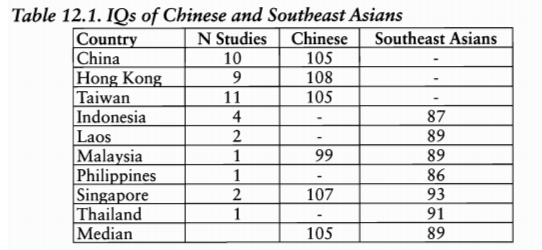
Chinese communities live throughout Southeast Asia (Cambodia, Indonesia, Malaysia, Philippines, Thailand, etc.). These small minorities are significantly more intelligent than Southeast Asians and socio-economically dominate the majority of indigenous populations. The Chinese are also called the “Jews of the East” by several sociologists. They also capture a very significant share of places in universities, as a result of which quotas and restrictions have been put in place against them in almost all South Asian countries. As in other multi-ethnic countries, the socio-economic hierarchy is dictated by IQ. East Asians form a distinct race (Chinese, Koreans, Japanese, etc.); their brain are larger than those of South-East Asians. They have a higher frequency of genes increasing intelligence, and their average IQ is significantly higher (105 compared to 89 for Southeast Asians). This 16-point difference is almost identical to the 15-point difference between African-Americans and Europeans in the USA. It explains Chinese domination.
In all Southeast Asian countries, the Chinese capture a share of wealth far greater than their proportion in the population. The ‘Control of Wealth’ in the table below indicates the share of capitalization of East Asian companies owned by Chinese. In Indonesia, for example, the Chinese are only 3.8% of the population but own 73% of the companies.
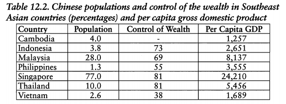
In Indonesia, the IQ difference between the indigenous and the Chinese is 18 points. The Chinese are much more intelligent and do better on university entrance tests. In 1982, the Indonesian government introduced quotas limiting the share of Chinese in universities to 6%. Southeast Asians with lower scores were admitted instead of Chinese (very similar to what happens in the USA with “positive discrimination,” allowing African-Americans and Hispanics to enter universities with lower scores than Europeans and East Asians).
Representing only 3.8% of Indonesia, the Chinese own 78% of the national wealth (Rigg, 2003). Similar figures have been given by Gooszen (2002), who estimates that in the first half of the twentieth century, the Chinese controlled 90% of the economy, while Mosher (2000) states that they owned 110 of the 140 largest corporate conglomerates.
In multiracial societies, successful minorities arouse envy, resentment, and frequently hatred from underperforming majorities. This can escalate into violence in which underperforming majorities attack, expropriate, or even kill higher IQ minorities. Throughout history, gentiles have persecuted Ashkenazi Jews, who with their high IQs have generally been successful and envious. The Chinese have attracted similar hostility in Indonesia. They were safe during the period of Dutch rule when law and order were maintained, but during the civil disorder of 1945-47 and the Indonesian takeover of political power, the Chinese were harassed in many ways. They were denied the property right. Confiscation and acquisition of their property was common, as was looting and pillaging; Chinese businessmen received “black bills” from Indonesian armed groups demanding huge sums. In 1945, there was extensive looting of Chinese and Eurasians; several hundred Chinese were killed. Twang Peck Yang (author of “The Chinese Business Elite in Indonesia and the Transition to Independence 1940-1950” 1998) explains that the Indonesian government opted for a socialist economy after independence because the ruling Indonesians realized that they “would probably lose to the Chinese in a free market economy” while “they could prosper in a controlled economy where large businesses were administered by the Indonesian government. In this way, the Indonesians who had political power were able to appoint their friends and relations and exclude the Chinese. ‘Thus, from 1945 onwards, a controlled economy was introduced in which large businesses were administered by the government while many Chinese businesses were destroyed and their business opportunities taken over, the Indonesian business class consolidated its position in domestic trade with the help of the state’ (Twang, 1998, p.163). Between 1945 and 1949, harassment of the Chinese increased, and a number of them left for Singapore. In 1965, widespread attacks on the Chinese left half a million dead and prompted tens of thousands to flee the country. There were further attacks on the Chinese in 1974 and 1998.
Candidates taking university entrance examinations in Indonesia were required to give their ethnic identity. To prevent the Chinese from trying to pass themselves off as indigenous Indonesians, “observers were instructed to examine their physical characteristics to confirm their racial self-identification” (Klitgaard, 1986, p. 121). The result of this discriminatory procedure was that several ethnic Chinese were rejected, while indigenous Indonesians with lower scores than the Chinese were admitted. Indonesia’s political elite operated a controlled economy to promote its advantage during the second half of the 20th century. In 1999, it was observed that “the Indonesian regulatory environment is characterized by bribery and other types of corruption. Many regulations are applied arbitrarily, and payments may be required to obtain ‘waivers’ from government regulation” (Johnson, Holmes, and Kirkpatrick 1999, p. 218). In a similar vein, the U.S. Department of Commerce (1998) reported that in the 1990s, “Indonesia continued to be a difficult place to do business; corruption is rife. The Chinese have fared much better economically in Indonesia than the indigenous peoples. How can this be explained? This question has often been asked. Perhaps Linda Lim (1997, 288) hints at the answer when they writes “The Chinese are the best endowed and most competitive members of the private sector.” What do they mean by best endowed? Is it possible that they suspect that the Chinese may be smarter than the Indonesians? If they harbor this suspicion, they have not developed it.
Cambodia gained independence in 1947. At that time, there was a Chinese minority that comprised 4% of the population. Nevertheless, “in the cities, retail trade is dominated by the Chinese, as are catering, hotels, export, import, and light manufacturing, including food processing, beverages, printing and machine shops; as much as 95% of the commercial class is Chinese; the wealthiest and most educated men during this period were Chinese (Pan, 1998, p. 146).
In Malaysia, just like in Indonesia, the high intelligence of the Chinese created resentment in the majority population. Quotas were established in 1980 by the Malaysian government to limit the massive over-representation of the Chinese in universities. A differential grading policy (!) was put in place. The Chinese and the Malays were thus graded separately in order to equalize the results of the two groups. Many Chinese went to study in Singapore, Australia, or England. The Malaysian government also imposed that 4/5 of public sector jobs be reserved for Malays.
In the Philippines, the first Chinese immigrants arrived around 1570. They quickly dominated economically. “The Chinese established new occupations and services, in addition to establishing a significant trade between China and the Philippines. They managed most of the trade, services, and intellectual occupations, quickly establishing a monopoly. The entire Spanish colony was economically dependent on the Chinese” (Wickberg, 1997, p.155). Manila’s Chinatown became “the business center of the entire city” (Wickberg, 1997, p. 159). In the second half of the 19th century, “the Spanish decided to make their colony in the Philippines profitable. One of the key measures was the unrestricted immigration of hard-working Chinese” (Wickberg, 1997). It also created a population of Filipino-Chinese hybrids who performed significantly better than the native Filipinos and formed, along with the pure Chinese, the elite. After independence in 1946, the government took steps to restrict the economic dominance of the Chinese (who owned 55% of the businesses while representing only 1.3% of the population) to give Filipinos more opportunities. Many Chinese migrants had not acquired citizenship, and the government restricted employment in many sectors to nationals only. The Chinese then moved into wholesale trade, light manufacturing, and financial services. They quickly dominated these sectors and “became more prosperous than ever” (Wickberg, 1997, p. 168). Edgar Wickberg, a leading scholar of the Philippines, wrote that “the Han Chinese outperformed the Filipinos in virtually every field.” Why? He offers no suggestions…
In Thailand, the Chinese represented 12% of the population in 1990. A community of Chinese traders has been present in Thailand since the 14th century. In Bangkok, the Chinese were the pioneers of the first publishing and press houses and cinemas. In 1987, a study was made of the 70 largest Thai companies. 67 were run by Chinese and only 3 by Thais. At the beginning of the 20th century, the Chinese owned the main banks, and “the king used Chinese capital and know-how to set up businesses”. In 1927, the Thai King Prajadhipok wrote a pamphlet entitled “Democracy in Siam,” which examined the advantages and disadvantages of introducing democracy. He first argued that the Chinese were more successful than the Thais in business: “there are many reasons why the Chinese can make money more quickly than other people. According to Chinese thought, money is the beginning and end of all good. The Chinese seem to want to do everything for money” (Reid, 1997, p. 5-6). He went on to argue that if democracy were introduced, the Chinese would inevitably take control of the country by applying the same motivations and skills that have made them dominant in business, and the parliament would be completely dominated by the Chinese. Even if the Chinese were excluded from all political rights, they would still dominate since they have the money. Any party that tried not to depend on Chinese funds could not succeed, so politics in Siam would be dominated and dictated by Chinese merchants (Tejapira, 1997, p. 80). He concluded that the best course was to keep political and military control of the country in Thai hands. As two American sociologists write, “the Chinese have been prosperous in Thailand for centuries” (Hamilton and Waters, 1997). As we have seen, throughout Southeast Asia, the indigenous people realized that they could not compete with the Chinese in a free society. Southeast Asians solved the problem by dictatorships or authoritarian regimes giving privileges to the indigenous people and discriminating against the Chinese. We have seen that this was the case in Indonesia, Malaysia, and the Philippines. It was also the case in Thailand, where, during the second half of the 20th century, the Chinese were banned from the officer ranks of the armed forces and had reduced voting rights and political candidacy rights (Tejapira, 1997).
The high achievement of East Asians throughout East Asia should not surprise us. It is identical to the high socio-economic and educational achievements of East Asians in Europe, the USA, Canada, Brazil, or Australia.
Conclusion
In whatever multiracial country in the world, the hierarchy remains remarkably unchanged (Africa, Australia, Brazil, England, Canada, Caribbean, Hawaii, Latin America, the Netherlands, New Zealand, Southeast Asia). Social sedimentation is dictated by intelligence. IQ is a physiological parameter essentially dictated by genes.
All data are available in The Global Bell Curve, 2009, Richard Lynn, Washington Summit Publishers.
